Fractional, Real, Imaginary and Complex Exponents #
When I was younger, I was told that exponentiation was repeated multiplication. I was also told that multiplication was repeated addition. I took this at face value and I though that this was how computers calculated things. It made sense for integers. It made sense that one could cheat repeated addition for powers of two by bit shifting and not repeated addition on platforms that only have addition, but not multiplication.
\[\begin{aligned} 2^5 & = 2 \times 2 \times 2 \times 2 \times 2 \\ 2^5 & = 2 + 2 + 2 + 2 \\ & + 2 + 2 + 2 + 2 \\ & + 2 + 2 + 2 + 2 \\ & + 2 + 2 + 2 + 2 \\ \end{aligned}\]Then I momentarily thought about square roots, because the square root of two can be written two ways:
\[\sqrt{2} = 2^{\frac{1}{2}}\]Using the mental framework with which my teachers had equiped me, meant that two is being multiplied by itself one-half times. This, of course, made no sense. How can one apply an operation a fractional amount of times? So then I wondered if looking at this in terms of addition would help, but that was a fractional amount too:
\[\begin{aligned} p & = b^m \\ p & = sb \\ sb & = b^m \\ s & = b^{m-1} \\ \end{aligned}\]Lets check our original example of \(2^5\)
\[\begin{aligned} m & = \log_2 2^5 = 5 \\ & \text{and} \\ s & = 2^{m-1} = 2^4 \\ \end{aligned}\]That checks out, but what about \(2^\frac{1}{2}\) ?
\[\begin{aligned} m & = \log_2 2^{\frac{1}{2}} = \frac{1}{2} \\ & \text{and} \\ s & = 2^{m-1} = 2^{-\frac{1}{2}} \\ \end{aligned}\]Of course, this is even more mystical because how does one apply addition ~0.707106 times? Fortunately, there’s a clue hidden in that \(\log_2\) function. But it’s not super obvious exactly how that helps us, at least not upon first glance. Don’t worry we’ll get there.
Logarithms #
Logarithms are interesting concept. Base ten logarithms let us know the magnitude of a decimal based number. A base two logarithm can let us know in which octave a frequency belongs. A base two logarithm can also let us know how many digits are needed to represent a number. Base two logarithms are found in measurements of entropy.
Mathematically, logarithms are pretty simple. They form a mapping from multiplication to addition:
\[\log(a^m) + \log(a^n) = \log(a^{m}a^{n})\]Additionally, they have the following relationships:
\[\begin{aligned} y & = b^x \text{, the exponential function in base b} \\ x & = \log_b y \text{, the logarithm in base b} \\ \end{aligned}\]Additionally, one can change the base of the logarithm simply by scaling the logarithm:
\[\log_{b_2} y = \frac{\log_{b_1} y}{\log_{b_1} b_2}\]Since, the base doesn’t matter, we can use the natural logarithm:
\[\log_{b_2} y = \frac{\ln y}{\ln b_2}\]The most commonly occuring logarithm is the natural logarithm, in base \(e\) :
\[\begin{aligned} x & = \ln e^x \\ \end{aligned}\]Using the identities above we can get:
\[\begin{aligned} y & = b^x \\ \log_{b} y & = \frac{\ln y}{\ln b} \\ \log_{b} y \ln b & = \ln y \\ x \ln b & = \ln y \\ e^{x \ln b} & = e^{\ln y} \\ e^{x \ln b} & = y \\ \end{aligned}\]This means that if we can figure out a way to compute \(\ln x\) and \(e^x\) for any value \(x\) , then we can compute any \(y = b^x\) by using \(y = e^{x \ln b}\) . Fortunately, using calculus we can figure out approximations for these functions. The process of doing so is called analytic continuation.
Analytic Continuation #
One of the most common introductions to the natural logarithm (besides the relationships and maps above), is the simple integral:
\[\ln(x) = \int_{1}^{x}\frac{dt}{t}\]This next graph is a combination of computing the area under the curve \(\frac{1}{x}\) from 1 to 2 along with \(\ln x\) , \(e^x\) , and \(x\) :
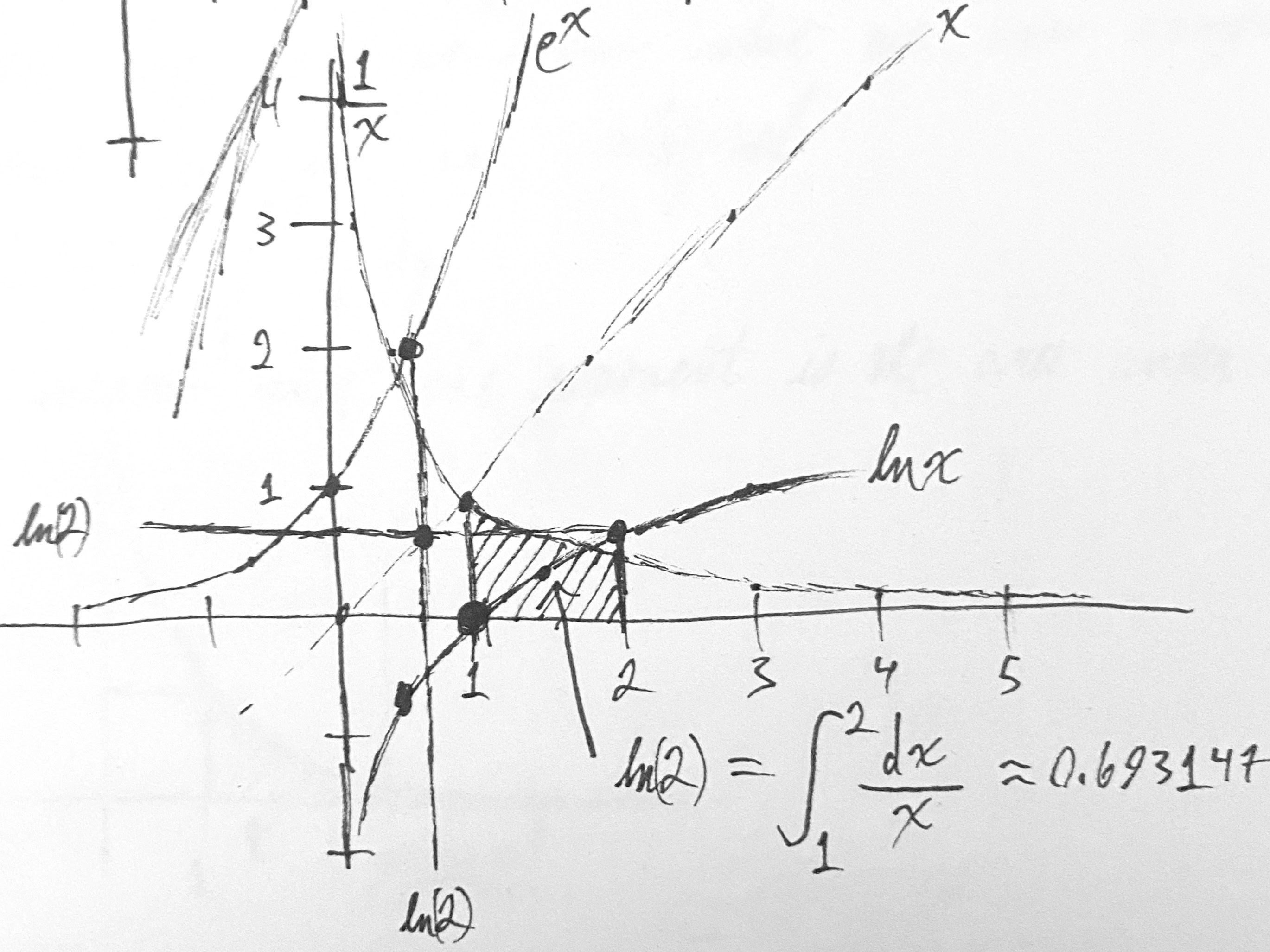
As should be obvious from the chart above, the exponential and the logarithm are inverses of each other are are reflections along the values of \(y = x\) . This means that if we can calculate one of these we can calculate both just by transposing the coordinate values.
There’s a problem with this though. The above integral definition of \(\ln\) is very limited in some important ways:
- It really can’t be extended into complex numbers, because the integral from \(1\) to \(a + b\imath\) is not defined without specifying an exact curve over which to integrate.
- The full integral needs to be computed, which limits its practicality in calculating a number to a certain precision within a small number of operations.
Fortunately, there are easily found analytic definitions for these functions using the method of Taylor series expansion. As an added benefit, these support imaginary and complex numbers in their domain:
\[\begin{aligned} e^x & = \sum_{k=0}^{\infty}\frac{x^k}{k!} \\ \ln x & = \sum_{k=1}^{\infty}\frac{(-1)^{k+1}}{k}(x-1)^k \\ \ln (1 + x) & = \sum_{k=1}^{\infty}{\frac{(-1)^{k-1}}{k}}x^{k} \end{aligned}\]There are some other identities that can come in handy because they tend to converge quickly. For when x falls with the complex unit circle:
\[\begin{aligned} \ln x & = 2\operatorname{artanh}\left(\frac{x-1}{x+1}\right) \\ & = \sum_{k=0}^{\infty}\frac{1}{2k+1}\left(\frac{x-1}{x+1}\right)^{2k+1} \end{aligned}\]When x is outside the complex unit circle:
\[\begin{aligned} \ln x & = 2\operatorname{arcoth}\left(\frac{x+1}{x-1}\right) \\ & = \sum_{k=0}^{\infty}\frac{1}{2k+1}\left(\frac{x+1}{x-1}\right)^{-(2k+1)} \end{aligned}\]There are some issues to be aware of around complex logarithms. To demonstrate these issues, we need Euler’s formula:
\[e^{\theta\imath} = \cos\theta +\imath\sin\theta \]Wait! We need a more complicated formula:
\[\begin{aligned} c^{a+b\imath} & = e^{c \ln a} e^{\imath c \ln b} \\ & = e^{c \ln a} \left( \cos (c \ln b) +\imath\sin (c \ln b) \right) \end{aligned}\]Since this has a periodic aspect to it, that means there are infinitely many loagrithms of a complex number. This is important to keep in mind, since some of the formulae above don’t seem to mind this. For instance those hyperbolic identities above only give what is called the “principle value”. This means the other infinitude of values are neglected, but can be computed from this.
Putting It All Together #
The analytic formulae all have summations between 0 or 1 and infinity. Computers don’t really like infinities because it takes them an infinite amount of time to deal with them. This means we’ve got to cheat. Cheating is easy: we just use a few terms of the analytic function. However, we still need to be mindful of the errors. The Taylor series really only has good accurracy for logarithms within a certain distance from the point we expanded the series around. In our case, that point is zero.
Since we know that the logarithm and exponential are realy the same thing just rotated around the the identity function, we can choose which ever one has the better convergence and then iteratively solve for a value using a variant of Newton’s method. In the case using the exponential, we just need to be careful of the large values generated in the factorials. Then we iteratively converge on the value we know while solving for the exponent.
Using everything we know about logarithms and exponents, we can set up a way to solve for \(\sqrt x\) :
\[\sqrt x = e^{\frac{1}{2}\ln x}\]Visually, we can see these relationships as:
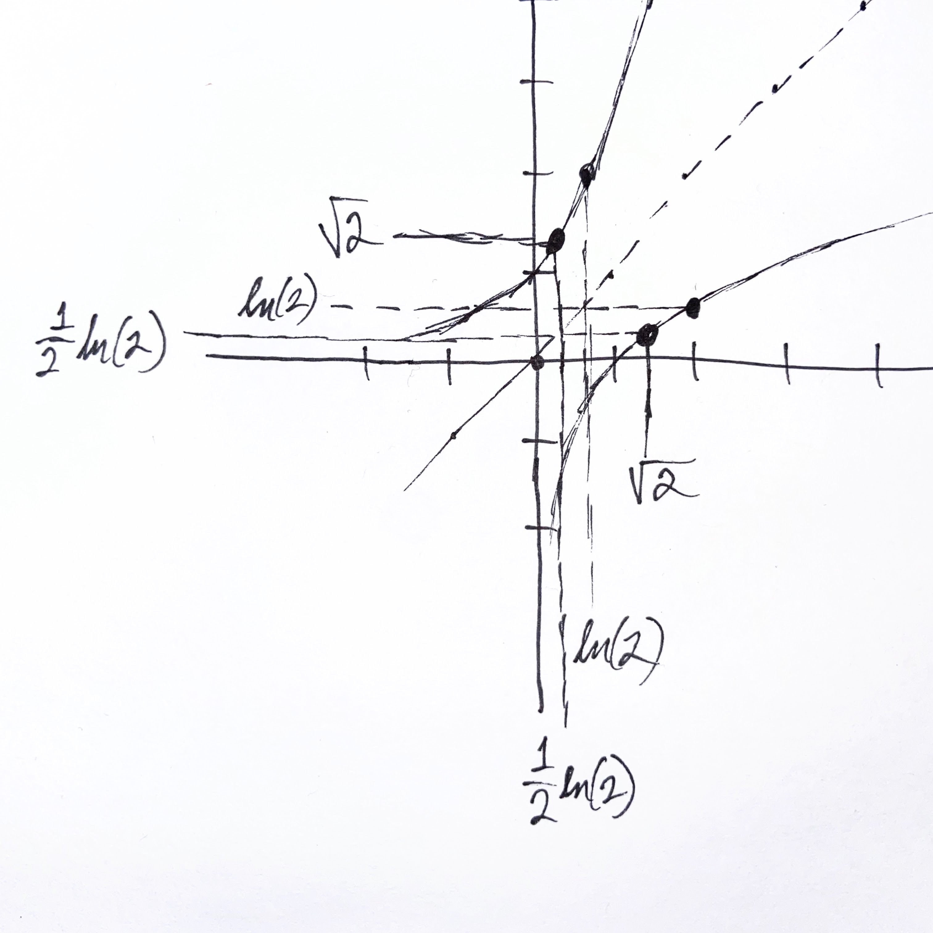
More generally, we can setup a general \(n^{th}\) root:
\[\sqrt[n] x = e^{\frac{1}{n}\ln x}\]This means we have found a general mechanism for performing \(n^{th}\) roots, or, more awkwardly, multiplying x by itself \(\frac{1}{n}\) times. But more than that, we have a general method for calculating roots, trigonometric functions, exponential and logarithmic functions themselves. Because of Euler’s formula, we can easily write:
\[\begin{aligned} \cos\theta & = \frac{e^{\theta\imath} + e^{-\theta\imath}}{2} \\ \sin\theta & = \frac{e^{\theta\imath} - e^{-\theta\imath}}{2\imath} \\ \tan \theta & = \frac{e^{\theta\imath} - e^{-\theta\imath}}{\imath(e^{\theta\imath} + e^{-\theta\imath})} \end{aligned}\]All of these methods arise from the relationships found in one particular equation:
\[b^x = e^{x \ln b}\]What Does This Mean? #
My preferred way of thinking about this, is integers are really a special case where our notational system happens to have the most simplicity for notating those numbers. They are points of minimal encoding, but they are just as complicated or information dense as any other algebraic number. This is how two infinite sums can be found in integer relationships to each other.
By asking the question I started with — “How do we multiply a number by itself a fractional number of times?” — we can find out new things about our numbers and operations. It is questions and answers like this which make me wonder what is more fundamental in terms of operations. Are fields with addition and groups with multiplication realy fundamental? Or is everything that we do really just an approximation or convergence of an infinity of terms reducing to a point for as long as it’s needed or convienient for our minds?
Is anything as simple as \(2+1\) ? Maybe it all is as complicated as: \[\begin{aligned} 2+1 & = e^{x \ln 2} \\ x & = \frac{\ln 2 + 1}{\ln 2} \\ 3 & = e^{\ln 2 + 1} \end{aligned}\]